This tutorial follows up on our previous one, where we introduced
SQL extensions in QuestDB
that make time series analysis easier. Today,
you will learn about the SAMPLE BY extension
in detail, which will enable you to work with time-series data efficiently
because of its simplicity and flexibility.
To get started with this tutorial, you should know that SAMPLE BY is a SQL
extension in QuestDB that helps you group or bucket time-series data based on
the designated timestamp. This removes
the need for lengthy CASE WHEN statements and GROUP BY clauses. Not only
that, the SAMPLE BY extension enables you to quickly deal with many other
data-related issues, such as
missing data,
incorrect timezones, and
offsets.
This tutorial assumes you have an up-and-running QuestDB instance ready for use. Let's dive straight into it.
Setup
Import sample data
Similar to the previous tutorial, we'll use the NYC taxi rides data for February 2018. You can use the following script that utilizes the HTTP REST API to upload data into QuestDB:
curl https://s3-eu-west-1.amazonaws.com/questdb.io/datasets/grafana_tutorial_dataset.tar.gz > grafana_data.tar.gz
tar -xvf grafana_data.tar.gz
curl -F data=@taxi_trips_feb_2018.csv http://localhost:9000/imp
curl -F data=@weather.csv http://localhost:9000/imp
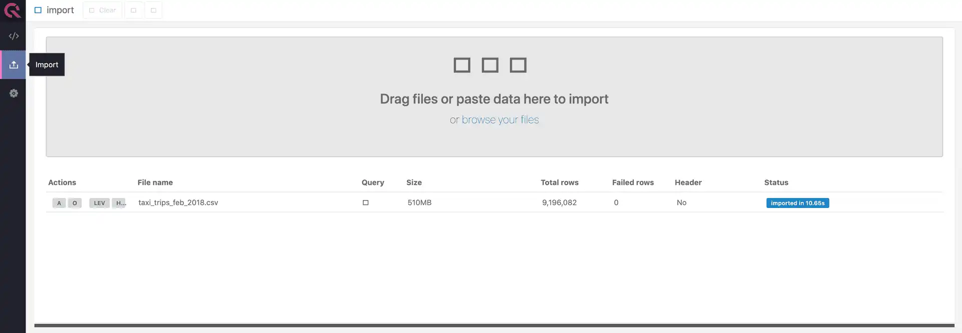
Alternatively, you can use the import functionality in the QuestDB console, as shown in the image below:
Create an ordered timestamp column
The SAMPLE BY keyword mandates the use of the
designated timestamp column to enable
further analysis. Therefore, you'll have to elect the pickup_datetime column
as the designated timestamp in a new table called taxi_trips with the script
below:
CREATE TABLE taxi_trips AS (
  SELECT *
    FROM "taxi_trips_feb_2018.csv"
   ORDER BY pickup_datetime
) TIMESTAMP(pickup_datetime)
PARTITION BY MONTH;
By converting the pickup_datetime column to timestamp, you are allowing
QuestDB to use it as the table's
designated timestamp. Using this
designated timestamp column, QuestDB is able to index the table to run
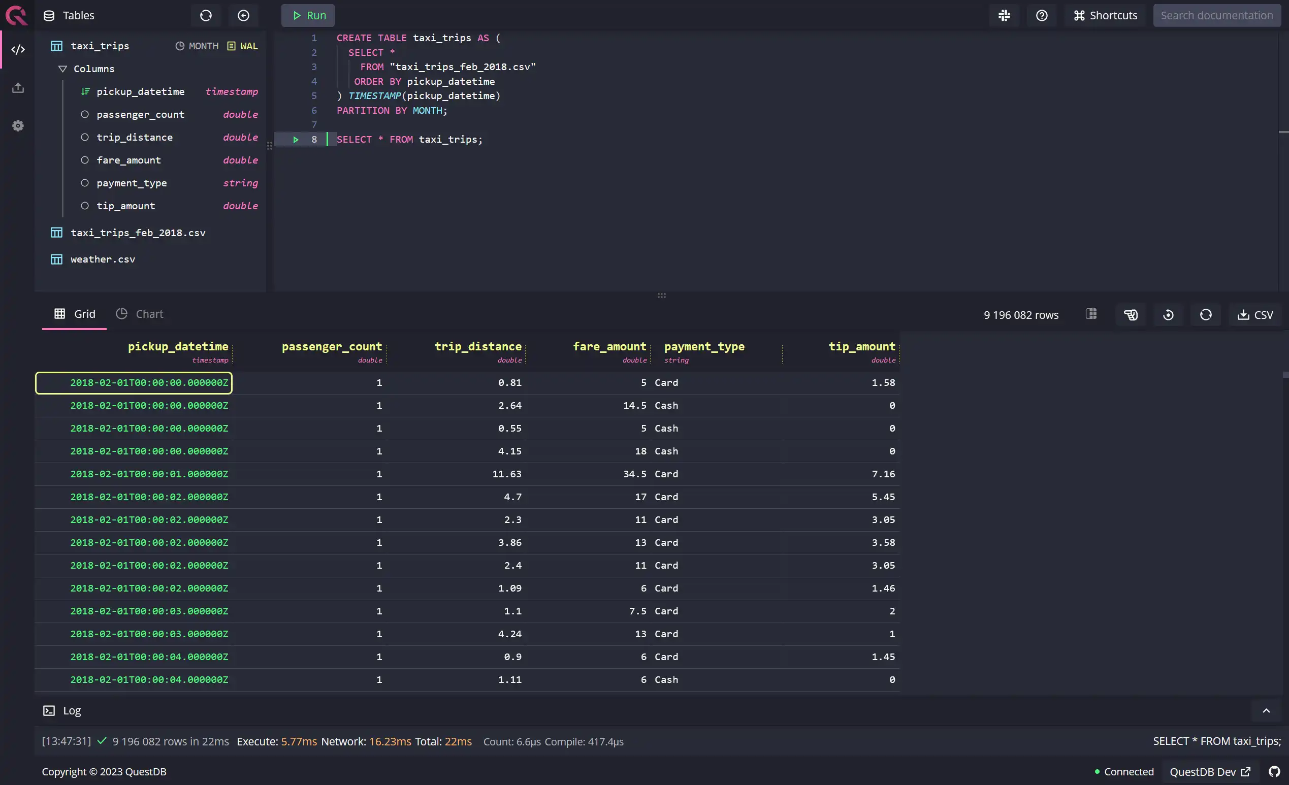
time-based queries more efficiently. If it all goes well, you should see the
following data after running a SELECT * query on the taxi_trips table:
Understanding the basics of SAMPLE BY
The SAMPLE BY extension allows you to create groups and buckets of data based
on time ranges. This is especially valuable for time-series data as you can
calculate frequently used aggregates with extreme simplicity. SAMPLE BY offers
you the ability to summarize or aggregate data from very fine to very coarse
units of time, i.e., from
microseconds to years and everything in between (milliseconds, seconds, minutes,
hours, days, and months). You can also derive other units of time, such as a
week or fortnight from the ones provided out of the box.
Let's look at some examples to understand how to use SAMPLE BY in different
scenarios.
Hourly count of trips
You can use the SAMPLE BY keyword with the
sample unit of h to get an
hour-by-hour count of trips for the whole duration of the data set. Running the
following query, you'll get results in the console:
SELECT
  pickup_datetime,
  COUNT() total_trips
FROM
  taxi_trips
SAMPLE BY 1h;
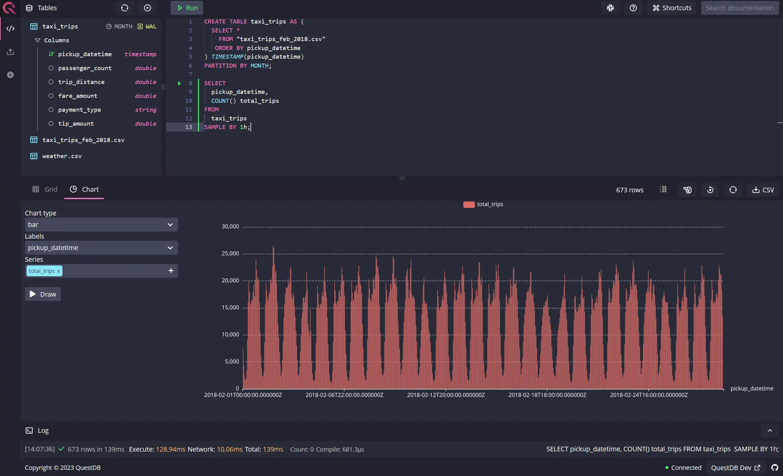
There are two ways you can read your data in the QuestDB console: using the grid, which has a tabular form factor, or using a chart, where you can draw up a line, bar, or an area chart to visualize your data. Here's an example of a bar chart drawn from the above query:
Three-hourly holistic summary of trips
The SAMPLE BY extension allows you to group data by any arbitrary number of
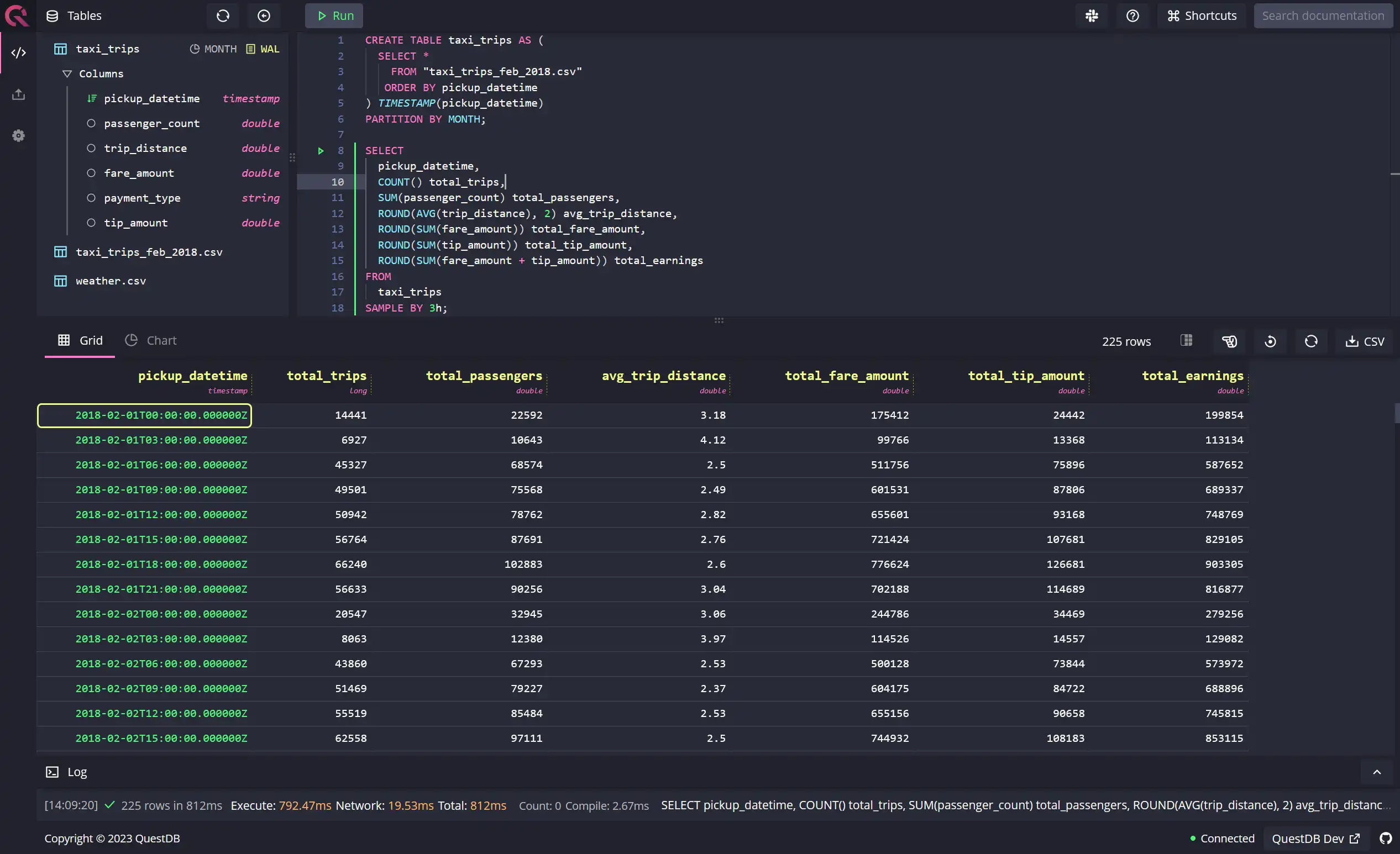
sample units. In the following example, you'll see that the query is calculating
a three-hourly summary of trips with multiple aggregate functions:
SELECT
  pickup_datetime,
  COUNT() total_trips,
  SUM(passenger_count) total_passengers,
  ROUND(AVG(trip_distance), 2) avg_trip_distance,
  ROUND(SUM(fare_amount)) total_fare_amount,
  ROUND(SUM(tip_amount)) total_tip_amount,
  ROUND(SUM(fare_amount + tip_amount)) total_earnings
FROM
  taxi_trips
SAMPLE BY 3h;
You can view the output of the query in the following grid on the QuestDB console:
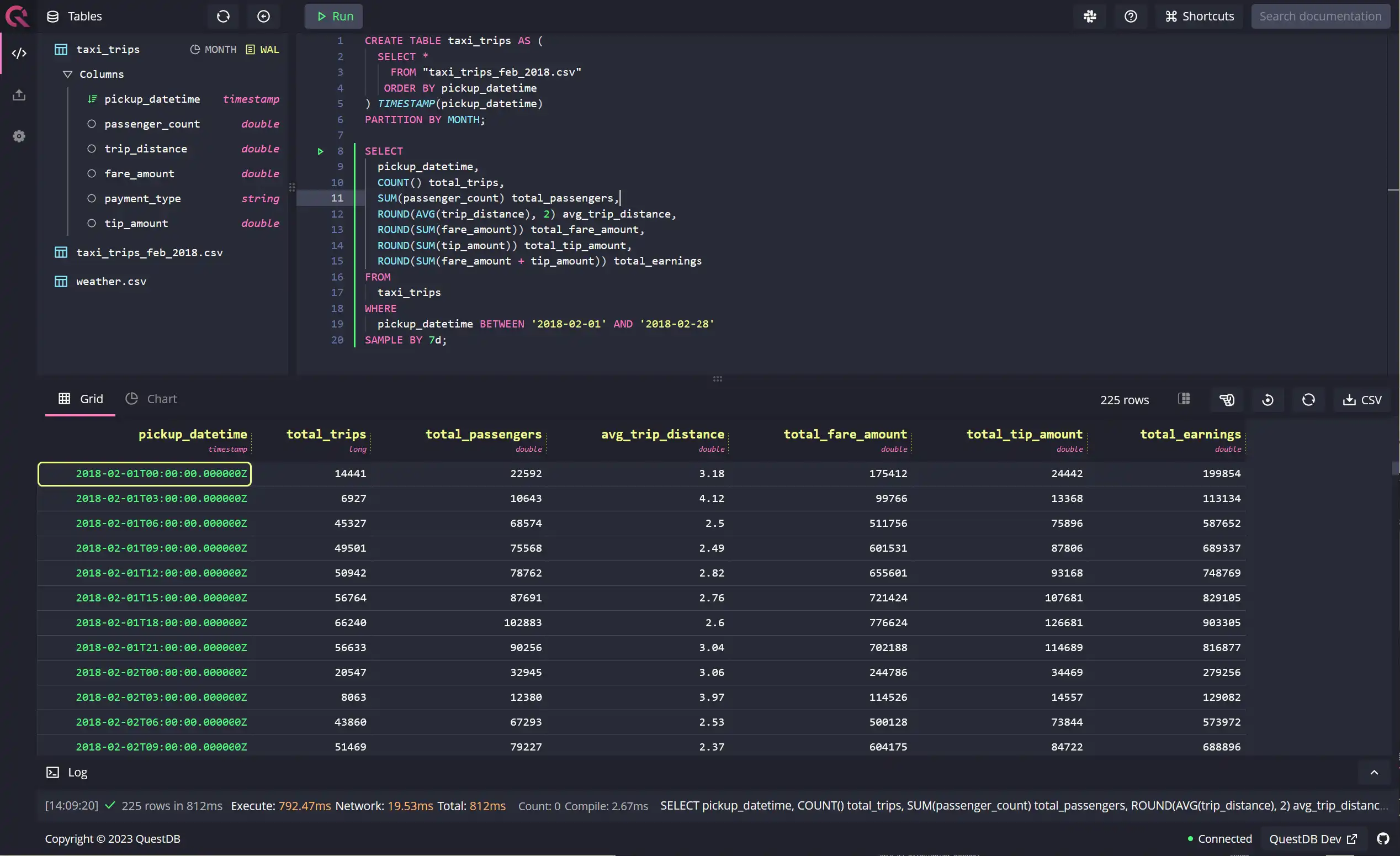
Weekly summary of trips
As mentioned above, although there's no sample unit for a week, or a fortnight,
you can derive them simply by utilizing the built-in sample units. If you want
to sample the data by a week, use 7d as the sampling time, as shown in the
query below:
SELECT
  pickup_datetime,
  COUNT() total_trips,
  SUM(passenger_count) total_passengers,
  ROUND(AVG(trip_distance), 2) avg_trip_distance,
  ROUND(SUM(fare_amount)) total_fare_amount,
  ROUND(SUM(tip_amount)) total_tip_amount,
  ROUND(SUM(fare_amount + tip_amount)) total_earnings
FROM
  taxi_trips
WHERE
  pickup_datetime BETWEEN '2018-02-01' AND '2018-02-28'
SAMPLE BY 7d;
Dealing with missing data
If you've worked a fair bit with data, you already know that data isn't always
in a pristine state. One of the most common issues, especially with time-series
data, is discontinuity, i.e., scenarios where data is missing for specific time
periods. You can quickly identify and deal with missing data using the advanced
functionality of the SAMPLE BY extension.
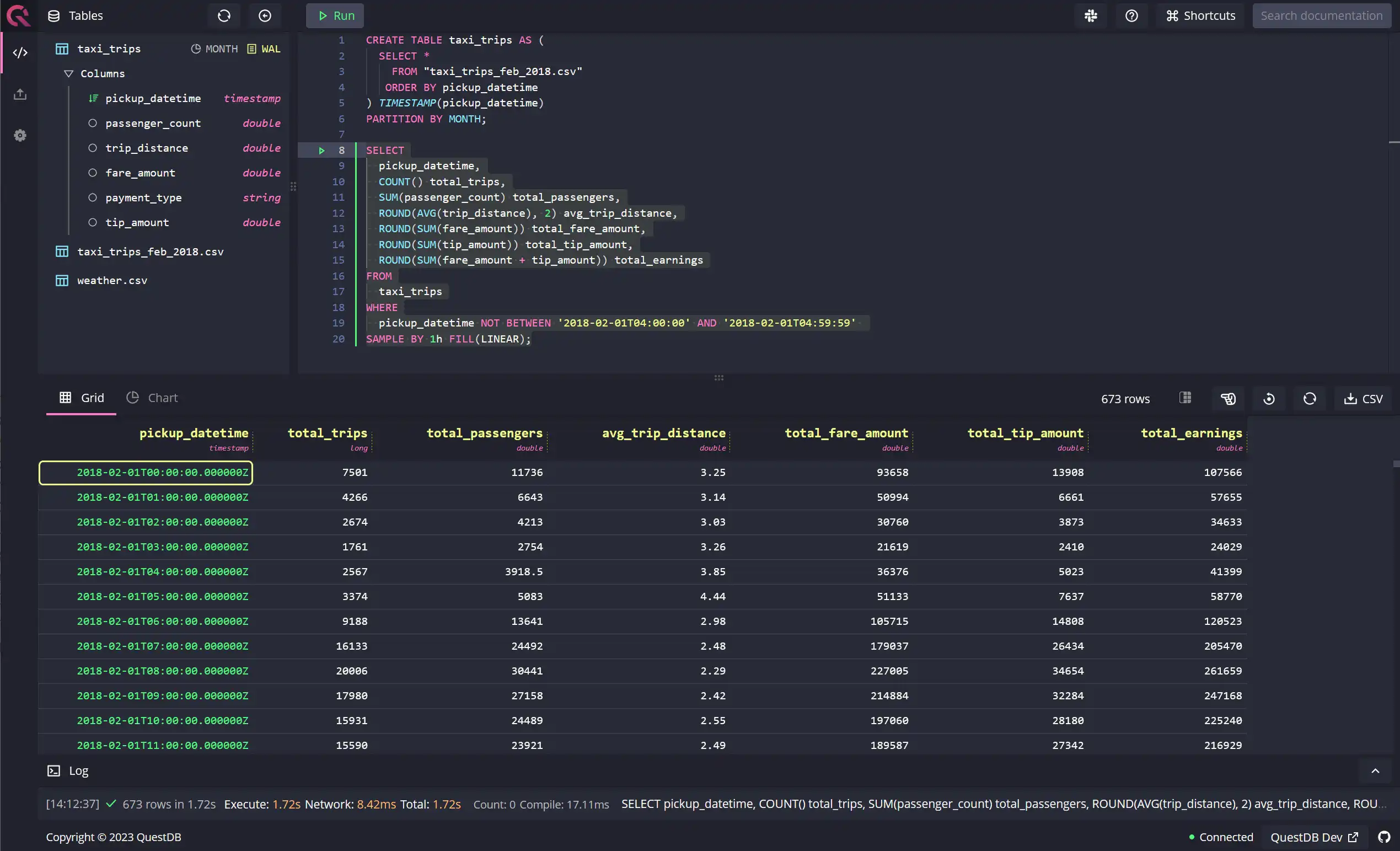
QuestDB offers an easy way to generate and fill in missing data with the
SAMPLE BY clause. Take the following example: I've deliberately removed data
from 4 am to 5 am for the 1st of February 2018. Notice how the
FILL keyword, when used in
conjunction with the SAMPLE BY extension, can generate a row for the hour
starting at 4 am and fill it with data generated from linear interpolation of
the 2 surrounding points:
SELECT
  pickup_datetime,
  COUNT() total_trips,
  SUM(passenger_count) total_passengers,
  ROUND(AVG(trip_distance), 2) avg_trip_distance,
  ROUND(SUM(fare_amount)) total_fare_amount,
  ROUND(SUM(tip_amount)) total_tip_amount,
  ROUND(SUM(fare_amount + tip_amount)) total_earnings
FROM
  taxi_trips
WHERE
  pickup_datetime NOT BETWEEN '2018-02-01T04:00:00' AND '2018-02-01T04:59:59'
SAMPLE BY 1h FILL(LINEAR);
The FILL keyword demands a
fillOption from the following:
fillOption | Usage scenario | Notes |
|---|---|---|
| NONE | When you don't want to populate missing data, and leave it as is | This is the default fillOption |
| NULL | When you want to generate rows for missing time periods, but leave all the values as NULLs | |
| PREV | When you want to copy the values of the previous row from the summarized data | This is useful when you expect the numbers to be similar to the preceding time period |
| LINEAR | When you want to normalize the missing values, you can take the average of the immediately preceding and following row | |
| CONST or x | When you want to hardcode values where data is missing | FILL (column_1, column_2, column_3, ...) |
Here's another example of hardcoding values using the FILL(x) fillOption:
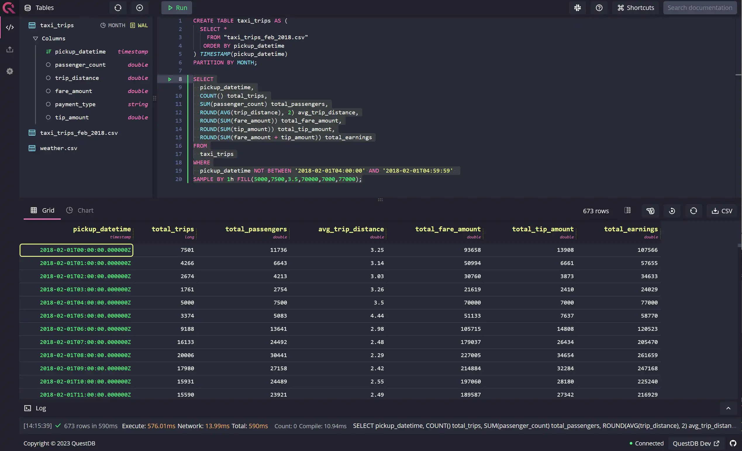
In the example above, we've used an inline WHERE clause to emulate missing
data with the help of the NOT BETWEEN keyword. Alternatively, you can create a
separate table with missing trips using the same idea, as shown below:
CREATE TABLE taxi_trips_missing AS (
  SELECT *
  FROM taxi_trips
  WHERE
    pickup_datetime NOT BETWEEN '2018-02-01T04:00:00' AND '2018-02-01T04:59:59'
);
Working with timezones and offsets
The SAMPLE BY extension also enables you to change timezones and add or
subtract offsets from your timestamp columns to adjust for any issues you might
encounter when dealing with different source systems, especially in different
geographic areas. It is important to note that, by default, QuestDB aligns its
sample calculation based on
the FIRST OBSERVATION, as shown in the example below:
SELECT
  pickup_datetime,
  COUNT() total_trips,
  SUM(passenger_count) total_passengers,
  ROUND(AVG(trip_distance), 2) avg_trip_distance,
  ROUND(SUM(fare_amount)) total_fare_amount,
  ROUND(SUM(tip_amount)) total_tip_amount,
  ROUND(SUM(fare_amount + tip_amount)) total_earnings
FROM
  taxi_trips
WHERE
  pickup_datetime BETWEEN '2018-02-01T13:35:52' AND '2018-02-28'
SAMPLE BY 1d;
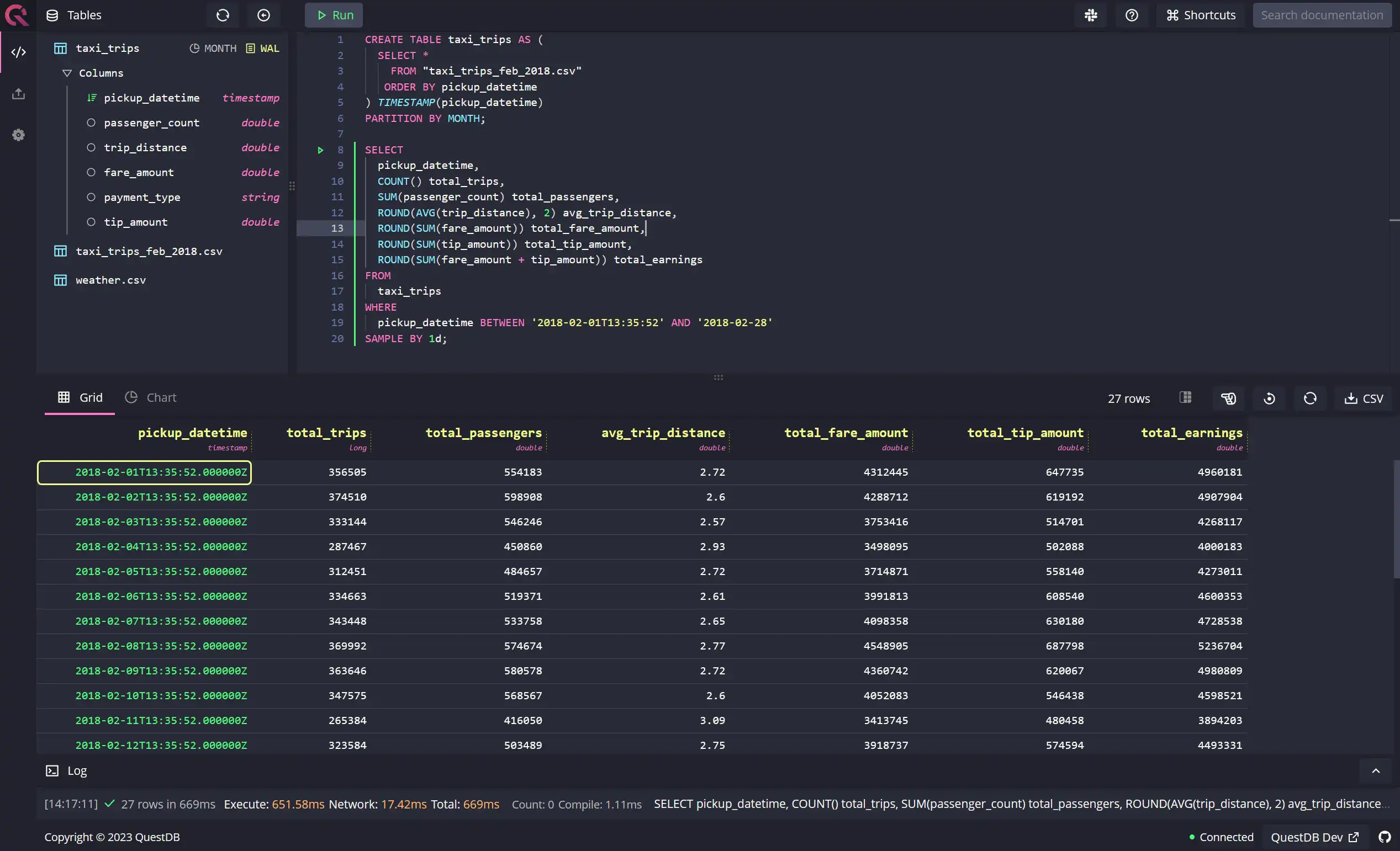
Note that now the 1d sample calculation starts at 13:35:52 and ends at
13:35:51 the next day. Apart from the option demonstrated above, there are two
other ways to align your sample calculations - to the
calendar time zone, and to
calendar with offset.
Let's take a look at the other two alignment methods.
Aligning sample calculation to another timezone
When moving data across systems, pipelines, and warehouses, you can encounter issues with time zones. For the sake of demonstration, let's assume that you're working in New York City, but you've identified that the timestamps of the data set you've loaded into the database are in Australian Eastern Time (instead of New York's EST). Traditionally, this could lead to extra conversion work to ensure that this new data is comparable to the rest of your data in EST.
QuestDB allows you to easily fix this issue by aligning your data to another
timezone using the
ALIGN TO CALENDAR TIME ZONE option
with the SAMPLE BY extension. In the example shown below, you can see how an
ALIGN TO CALENDAR TIME ZONE ('AEST') has aligned the pickup_datetime, i.e.,
the designated timestamp column to the AEST timezone for Melbourne.
SELECT
  pickup_datetime,
  COUNT() total_trips,
  SUM(passenger_count) total_passengers,
  ROUND(AVG(trip_distance), 2) avg_trip_distance,
  ROUND(SUM(fare_amount)) total_fare_amount,
  ROUND(SUM(tip_amount)) total_tip_amount,
  ROUND(SUM(fare_amount + tip_amount)) total_earnings
FROM
  taxi_trips
SAMPLE BY 3h ALIGN TO CALENDAR TIME ZONE ('AEST');

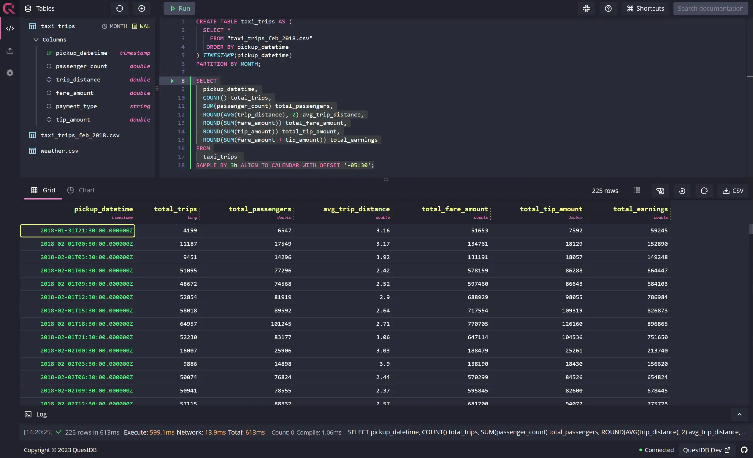
Aligning sample calculation with offsets
Similar to the previous example, you can also align the sample calculation by
offsetting the designated timestamp
column manually by any hh:mm value between -23:59 to 23:59. In the following
example, we're offsetting the sample calculation by -5:30, i.e., negative five
hours and thirty minutes:
SELECT
  pickup_datetime,
  COUNT() total_trips,
  SUM(passenger_count) total_passengers,
  ROUND(AVG(trip_distance), 2) avg_trip_distance,
  ROUND(SUM(fare_amount)) total_fare_amount,
  ROUND(SUM(tip_amount)) total_tip_amount,
  ROUND(SUM(fare_amount + tip_amount)) total_earnings
FROM
  taxi_trips
SAMPLE BY 3h ALIGN TO CALENDAR WITH OFFSET '-05:30';
Conclusion
In this tutorial, you learned how to exploit the
SAMPLE BY extension in QuestDB to work
efficiently with time-series data, especially in aggregated form. In addition,
the SAMPLE BY extension also allows you to fix common problems with
time-series data attributable to complex data pipelines, disparate source
systems in different geographical areas, software bugs, etc. All in all, SQL
extensions in QuestDB, like SAMPLE BY, provide a significant advantage when
working with time-series data by enabling you to achieve more in fewer lines of
SQL.